Quantification of follow-up: code accompanying paper

Author

Kaspar Rufibach, on behalf of the follow-up quantification taks force of the oncology estimand WG

Published

April 14, 2023

1 Background

Code for the paper Rufibach et al. (2023) (download from journal, download from arxiv) written by the follow-up quantification task force of the oncology estimand WG.

2 Purpose of this document

This R markdown file provides easy accessible code to compute all the quantifiers for follow-up. The github repository where this document is hosted is available here.

To illustrate the functions all clinical trial data in this file is simulated. In the paper, the PH examples uses real data.

3 Setup

3.1 Packages

# --------------------------------------------------------------
# packages
# --------------------------------------------------------------
packs <- c("survival", "rpact", "survRM2")    
for (i in 1:length(packs)){library(packs[i], character.only = TRUE)}

3.2 Functions

Below all functions are defined.

quantifyFU: This function provides all the seven methods described in the paper draft.
plot.qfu: Plot the distributions from which medians are computed.

# --------------------------------------------------------------
# functions
# --------------------------------------------------------------

# function to compute all the different variants of follow-up quantification
quantifyFU <- function(rando, event_time, event_type, ccod){
  
  ## =================================================================
  ## compute all FU measures
  ## =================================================================

  # input arguments:
  # - rando: date of randomization
  # - event_time: time to event or time to censoring
  # - event_type: 0 = event, 1 = lost to FU, 2 = administratively censored
  # - ccod: clinical cutoff date

  require(survival)

  n <- length(rando)

  # objects to collect distributions
  res <- NULL
  
  # indicator for lost to follow up
  ltfu_cens <- as.numeric(event_type == 1)

  # indicator for administratively censored
  admin_cens <- as.numeric(event_type == 2)

  # usual censoring indicator: 0 = censored (for whatever reason), 1 = event
  primary_event <- as.numeric(event_type == 0)

  # indicator for censoring
  event_time_cens <- as.numeric(primary_event == 0)

  # observation time regardless of censoring
  ecdf1 <- as.list(environment(ecdf(event_time)))
  res[[1]] <- cbind(ecdf1$x, 1 - ecdf1$y)
  m1 <- median(event_time)
  
  # observation time for those event-free
  d2 <- event_time[event_time_cens == 1]
  ecdf2 <- as.list(environment(ecdf(d2)))
  res[[2]] <- cbind(ecdf2$x, 1 - ecdf2$y)
  m2 <- median(d2)

  # time to censoring
  so3 <- survfit(Surv(event_time, event_time_cens) ~ 1)
  res[[3]] <- so3
  m3 <- summary(so3)$table["median"]

  # time to CCOD, potential followup
  pfu <- as.numeric((ccod - rando) / 365.25 * 12)
  ecdf4 <- as.list(environment(ecdf(pfu)))
  res[[4]] <- cbind(ecdf4$x, 1 - ecdf4$y)
  m4 <- median(pfu)
  
  # known function time
  m5 <- rep(NA, n)
  m5[event_time_cens == 1] <- event_time[event_time_cens == 1]
  m5[primary_event == 1] <- pfu[primary_event == 1]
  ecdf5 <- as.list(environment(ecdf(m5)))
  res[[5]] <- cbind(ecdf5$x, 1 - ecdf5$y)
  m5 <- median(m5)
  
  # Korn's potential follow-up time
  spfu <- sort(pfu)
  pt <- rep(NA, n)
  for (i in 1:n){
  
    # timepoint at which we compute potential followup (t' in Schemper et al)
    t <- spfu[i]
  
    # proportion with pfu > t
    pet <- mean(spfu > t)
  
    # time to LTFU
    so6 <- survfit(Surv(event_time, ltfu_cens) ~ 1, subset = (pfu >= t))
    pltet <- ifelse(max(so6$time > t) == 0, 0, so6$surv[so6$time > t][1])
  
    pt[i] <- pltet * pet
  }

  res[[6]] <- cbind(spfu, pt)
  
  # now take the median of the distribution, see plot(t, pt, type = "s")
  m6 <- max(spfu[pt >= 0.5])

  # Potential follow-up considering events
  m7 <- rep(NA, n)
  m7[event_time_cens == 1] <- pfu[event_time_cens == 1]
  m7[primary_event == 1] <- event_time[primary_event == 1]
  ecdf7 <- as.list(environment(ecdf(m7)))
  res[[7]] <- cbind(ecdf7$x, 1 - ecdf7$y)
  m7 <- median(m7)

  # summarize results for medians
  dat <- matrix(NA, nrow = 7, ncol = 1)
  dat[, 1] <- c(m1, m2, m3, m4, m5, m6, m7)
  rownames(dat) <- c("Observation time regardless of censoring", 
                     "Observation time for those event-free", 
                     "Time to censoring", "Time to CCOD", 
                     "Known function time", "Korn potential follow-up", 
                     "Potential follow-up considering events")
  colnames(dat) <- "median"
  
  output <- list("medians" = dat, "distributions" = res)
  class(output) <- "qfu"
  return(output)
}

# function to plot distributions of various quantifiers
plot.qfu <- function(x, which = 1:7, median = TRUE){
  
  dat <- x$distributions
  
  par(las = 1)
  plot(0, 0, type = "n", xlim = c(0, 1.05 * max(dat[[1]][, 1])), ylim = c(0, 1), 
       xlab = "time-to-event endpoint", ylab = "probability", 
       main = "Distributions used for quantification of follow-up")
  if (3 %in% which){lines(dat[[3]], col = 3, conf.int = FALSE)}
  which <- which[which != 3]
  for (i in which){lines(dat[[i]], col = i)}
  
  if(isTRUE(median)){abline(h = 0.5, col = grey(0.5), lwd = 2)}
  
  legend("bottomleft", rownames(x$medians)[which], lty = 1, 
         col = (1:7)[which], bty = "n", lwd = 2)
}

# compute value of KM estimate and CI
confIntKM_t0 <- function(time, event, t0, conf.level = 0.95){

  alpha <- 1 - conf.level

  # compute ci according to the formulas in Huesler and Zimmermann, Chapter 21
  obj <- survfit(Surv(time, event) ~ 1, conf.int = 1 - alpha, conf.type = "plain", 
                 type = "kaplan", error = "greenwood", conf.lower = "peto")
  St <- summary(obj)$surv
  t <- summary(obj)$time
  n <- summary(obj)$n.risk
  res <- matrix(NA, nrow = length(t0), ncol = 3)

  for (i in 1:length(t0)){
    ti <- t0[i]
    if (min(t) > ti){res[i, ] <- c(1, NA, NA)}
    if (min(t) <= ti){    
        if (ti %in% t){res[i, ] <- rep(NA, 3)} else {
            Sti <- min(St[t < ti])
            nti <- min(n[t < ti])        
            Var.peto <- Sti ^ 2 * (1 - Sti) / nti
            Cti <- exp(qnorm(1 - alpha / 2) * sqrt(Var.peto) / 
                         (Sti ^ (3 / 2) * (1 - Sti)))
            ci.km <- c(Sti / ((1 - Cti) * Sti + Cti), Cti * Sti / 
                         ((Cti - 1) * Sti + 1))
            res[i, ] <- c(Sti, ci.km)}
    } # end if
  } # end for

  res <- cbind(t0, res)
  dimnames(res)[[2]] <- c("t0", "S at t0", "lower.ci", "upper.ci")
  return(res)
}

# bootstrap survival data
bootSurvivalSample <- function(surv.obj, n, M = 1000, track = TRUE){
     
     # bootstrap right-censored survival data according to Efron (1981)
     # see Akritas (1986) for details
     # surv.obj: Surv object to sample from
     # n: sample size for samples to be drawn
     # M: number of samples
     
     n.surv <- nrow(surv.obj)
     res.mat <- data.frame(matrix(NA, ncol = M, nrow = n))
     
     for (i in 1:M){
          ind <- sample(1:n.surv, size = n, replace = TRUE)
          res.mat[, i] <- surv.obj[ind]
          if (track){print(paste("sample ", i, " of ", M, " done", sep = ""))}
     }
     
     return(res.mat)
}

# compute value and CI for difference of survival probabilities at milestone, 
# via bootstrap
confIntMilestoneDiff <- function(time, event, group, t0, M = 10 ^ 3, 
                                 conf.level = 0.95){
  
  ind <- (group == levels(group)[1])
  s.obj1 <- Surv(time[ind], event[ind])
  s.obj2 <- Surv(time[!ind], event[!ind])
  n1 <- sum(ind)
  n2 <- sum(!ind)
  
  res1 <- bootSurvivalSample(surv.obj = s.obj1, n = n1, M = M, track = FALSE)
  res2 <- bootSurvivalSample(surv.obj = s.obj2, n = n2, M = M, track = FALSE)
  
  boot.diff1 <- rep(NA, M)
  boot.diff2 <- boot.diff1
  
  for (i in 1:M){
    
    # based on KM
    t1km <- confIntKM_t0(time = as.matrix(res1[, i])[, "time"], event = 
                           as.matrix(res1[, i])[, "status"], t0, conf.level = 0.95)[2]
    t2km <- confIntKM_t0(time = as.matrix(res2[, i])[, "time"], event = 
                           as.matrix(res2[, i])[, "status"], t0, conf.level = 0.95)[2]
    boot.diff1[i] <- t1km - t2km
    
    # based on exponential fit
    r1 <- exp(- coef(survreg(res1[, i] ~ 1, dist = "exponential")))
    t1 <- 1 - pexp(t0, rate = r1)
    
    r2 <- exp(- coef(survreg(res2[, i] ~ 1, dist = "exponential")))
    t2 <- 1 - pexp(t0, rate = r2)
    
    boot.diff2[i] <- t1 - t2 
    
  }
  
  # from bootstrap sample of differences just take symmetric quantiles to get 
  # CI for difference
  alpha <- 1 - conf.level
  ci1 <- quantile(boot.diff1, probs = c(alpha / 2, 1 - alpha / 2), na.rm = TRUE)
  ci2 <- quantile(boot.diff2, probs = c(alpha / 2, 1 - alpha / 2), na.rm = TRUE)
  
  res <- list("km" = ci1, "exponential" = ci2)
  return(res)
}

# compute the extreme limits as described by Betensky
stabilityKM <- function(time, event){
  
  ind <- (event == 0)
  maxevent <- max(time[event == 1])
  
  # extreme scenarios (not precisely) according to Betensky (2015)
  # lower bound: every censored patient has event at censoring date
  t_low <- time
  c_low <- event
  c_low[ind] <- 1

  # upper bound: every censored observation has censoring time equal 
  # to maximum event time 
  t_up <- time
  t_up[ind & (time < maxevent)] <- maxevent
  c_up <- event

  # collect results
  res <- list("t_low" = t_low, "c_low" = c_low, "t_up" = t_up, "c_up" = c_up)
  return(res)
}

4 Example: Proportional hazards

4.1 Simulate a clinical trial with time-to-event endpoint using `rpact`

A clinical trial with very similar properties as the Gallium data in Rufibach et al. (2022) is simulated using rpact Wassmer and Pahlke (2021).

# simulate a clinical trial using rpact
# time unit is months
design <- getDesignGroupSequential(informationRates = 1,
   typeOfDesign = "asOF", sided = 1, alpha = 0.025, beta = 0.2)

simulationResult <- getSimulationSurvival(design,
    lambda2 = log(2) / 60, hazardRatio = 0.75,
    dropoutRate1 = 0.025, dropoutRate2 = 0.025, 
    dropoutTime = 12,
    accrualTime = 0:6, 
    accrualIntensity = 6 * 1:7,
    plannedEvents = 350,
    directionUpper = FALSE,
    maxNumberOfSubjects = 1000,
    maxNumberOfIterations = 1,
    maxNumberOfRawDatasetsPerStage = 1,
    seed = 2021)

# retrieve dataset
simdat <- getRawData(simulationResult)

# create variable with randomization dates
# note that addition / subtraction of date objects happens in days 
# --> multiplication by 365.25 / 12 ~= 30 below
day0 <- as.Date("2016-01-31", origin = "1899-12-30")
rando <- day0 + simdat$accrualTime * 365.25 / 12
pfs <- simdat$timeUnderObservation

# event type variable: 0 = event, 1 = lost to FU, 2 = administratively censored
event_type <- rep(NA, nrow(simdat))
event_type[simdat$event == TRUE] <- 0
event_type[simdat$event == FALSE & simdat$dropoutEvent == TRUE] <- 1
event_type[simdat$event == FALSE & simdat$dropoutEvent == FALSE] <- 2 

# PFS event
pfsevent <- as.numeric(event_type == 0)

# treatment arm
arm <- factor(simdat$treatmentGroup, levels = 1:2, labels = c("G", "R"))

# define clinical cutoff date based on simulation result
ccod <- day0 + simdat$lastObservationTime[1] * 365.25 / 12
  
# check
so1 <- summary(coxph(Surv(pfs, pfsevent) ~ arm))
so1

Call:
coxph(formula = Surv(pfs, pfsevent) ~ arm)

  n= 1000, number of events= 350 

       coef exp(coef) se(coef)     z Pr(>|z|)  
armR 0.2351    1.2650   0.1073 2.191   0.0285 *
---
Signif. codes:  0 '***' 0.001 '**' 0.01 '*' 0.05 '.' 0.1 ' ' 1

     exp(coef) exp(-coef) lower .95 upper .95
armR     1.265     0.7905     1.025     1.561

Concordance= 0.528  (se = 0.014 )
Likelihood ratio test= 4.82  on 1 df,   p=0.03
Wald test            = 4.8  on 1 df,   p=0.03
Score (logrank) test = 4.82  on 1 df,   p=0.03

Plot the Kaplan-Meier estimates:

par(las = 1)
plot(survfit(Surv(pfs, pfsevent) ~ arm), col = 2:3, mark = "'", lty = 1, xlim = c(0, 100), 
     xlab = "PFS", ylab = "probability of being event-free")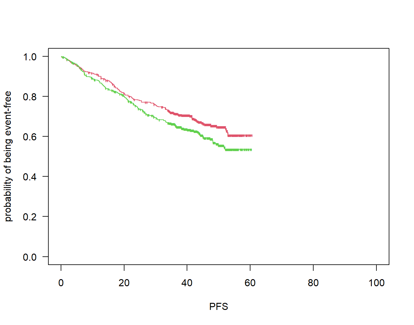

4.2 Precision

Compute survival probabilities, their differences and confidence intervals at milestones.

ms <- c(36, 48)
msR1 <- confIntKM_t0(time = pfs[arm == "R"], event = pfsevent[arm == "R"], t0 = ms, 
                     conf.level = 0.95)
msG1 <- confIntKM_t0(time = pfs[arm == "G"], event = pfsevent[arm == "G"], t0 = ms, 
                     conf.level = 0.95)
msR1

     t0   S at t0  lower.ci  upper.ci
[1,] 36 0.6625629 0.6054758 0.7152741
[2,] 48 0.5870704 0.4922056 0.6758830

msG1

     t0   S at t0  lower.ci  upper.ci
[1,] 36 0.7149897 0.6622073 0.7624827
[2,] 48 0.6536542 0.5662833 0.7317616

# differences
ms1d1 <- confIntMilestoneDiff(time = pfs, event = pfsevent, group = arm, 
                             t0 = ms[1], M = 10 ^ 3, conf.level = 0.95)$km
ms2d1 <- confIntMilestoneDiff(time = pfs, event = pfsevent, group = arm, 
                              t0 = ms[2], M = 10 ^ 3, conf.level = 0.95)$km
ms1d1

        2.5%        97.5% 
-0.003376164  0.114936362

ms2d1

         2.5%         97.5% 
-0.0007250327  0.1350419043

4.3 Quantification of follow-up using various methods

Now let us apply the above functions:

fu <- quantifyFU(rando = rando, event_time = pfs, event_type = event_type, ccod = ccod)

# medians of all these distributions:
fu$medians

                                           median
Observation time regardless of censoring 38.28363
Observation time for those event-free    42.87887
Time to censoring                        44.05744
Time to CCOD                             45.78363
Known function time                      44.55744
Korn potential follow-up                 44.15268
Potential follow-up considering events   40.31934

Plot distributions:

plot(fu)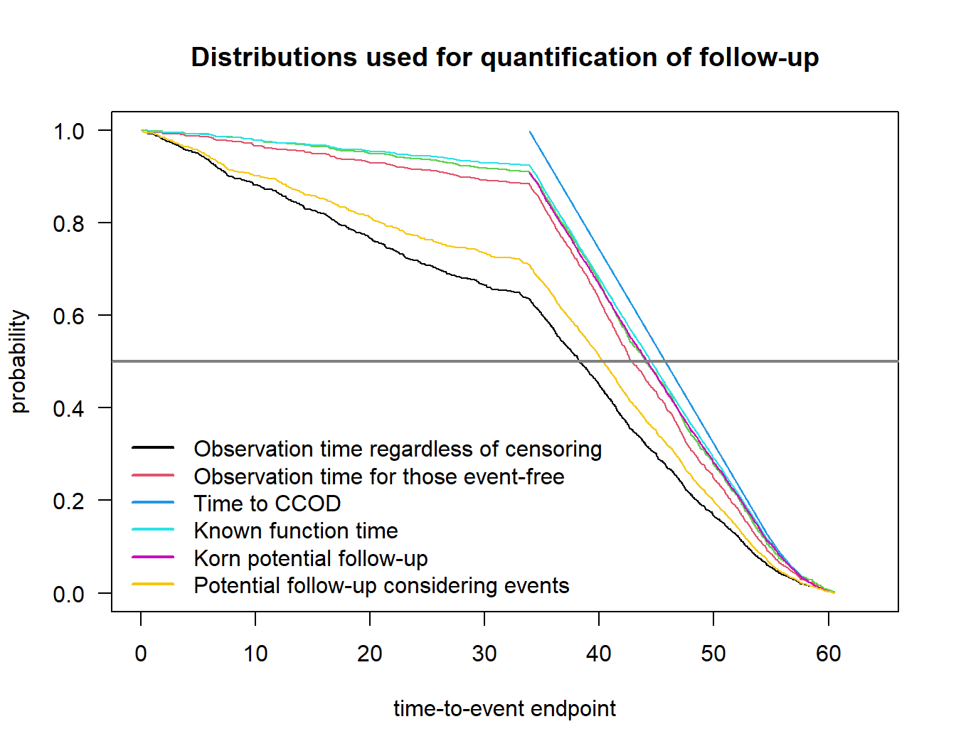

5 Example: delayed separation

5.1 Simulate a clinical trial with time-to-event endpoint using `rpact`

# Simulation assuming a delayed treatment effect
alpha <- 0.05
beta <- 0.2
design <- getDesignGroupSequential(informationRates = 1, typeOfDesign = "asOF", sided = 1, 
                                   alpha = alpha / 2, beta = beta)

piecewiseSurvivalTime <- c(0, 12)
baserate <- log(2) / 60
hr_nph <- 0.65
dropoutRate <- 0.025
dropoutTime <- 12
accrualTime <- 0:6
accrualIntensity <- 6 * 1:7
plannedEvents <- 389
maxNumberOfSubjects <- 1000
maxNumberOfIterations <- 10 ^ 3

simulationResultNPH <- getSimulationSurvival(design,
                           piecewiseSurvivalTime = piecewiseSurvivalTime,
                           lambda2 = c(baserate, baserate),
                           lambda1 = c(baserate, hr_nph * baserate),
                           dropoutRate1 = dropoutRate, 
                           dropoutRate2 = dropoutRate, dropoutTime = dropoutTime,
                           accrualTime = accrualTime, 
                           accrualIntensity = accrualIntensity,
                           plannedEvents = plannedEvents,
                           directionUpper = FALSE,
                           maxNumberOfSubjects = maxNumberOfSubjects,
                           maxNumberOfIterations = maxNumberOfIterations,
                           maxNumberOfRawDatasetsPerStage = 10 ^ 4,
                           seed = 2021)

# power for logrank test
simulationResultNPH$overallReject

[1] 0.805

# access raw simulation data
simdat <- getRawData(simulationResultNPH)

# extract simulation run 1 for example in paper
simpick <- 1
simdat_run1 <- subset(simdat, iterationNumber == simpick)

# median time-to-dropout
med_do <- - log(2) / log((1- dropoutRate)) * dropoutTime

# create variable with randomization dates
# note that addition / subtraction of date objects happens in days 
# --> multiplication by 365.25 / 12 ~= 30 below
day0_nph <- as.Date("2016-01-31", origin = "1899-12-30")
rando_nph <- day0_nph + simdat_run1$accrualTime * 365.25 / 12
pfs1_nph <- simdat_run1$timeUnderObservation

# event type variable: 0 = event, 1 = lost to FU, 
# 2 = administratively censored
event_type_nph <- rep(NA, nrow(simdat_run1))
event_type_nph[simdat_run1$event == TRUE] <- 0
event_type_nph[simdat_run1$event == FALSE & 
                 simdat_run1$dropoutEvent == TRUE] <- 1
event_type_nph[simdat_run1$event == FALSE & 
                 simdat_run1$dropoutEvent == FALSE] <- 2 

# PFS event
pfsevent1_nph <- as.numeric(event_type_nph == 0)

# treatment arm
arm_nph <- factor(simdat_run1$treatmentGroup, levels = 1:2, labels = c("G", "R"))

# define clinical cutoff date based on simulation result
ccod1_nph <- day0_nph + simdat_run1$lastObservationTime[1] * 365.25 / 12

Plot Kaplan-Meier estimates:

par(las = 1, mar = c(4.5, 4.5, 2, 1), oma = c(0, 0, 3, 0))

so1_nph <- survfit(Surv(pfs1_nph, pfsevent1_nph) ~ arm_nph)
plot(so1_nph, col = 2:3, mark = "'", lty = 1, xlim = c(0, 100), xlab = "PFS (months)", 
     ylab = "probability of not having a PFS event")

abline(v = ms, col = grey(0.5), lwd = 2, lty = 2)

# title
mtext("Delayed separation", 3, line = 0, outer = TRUE)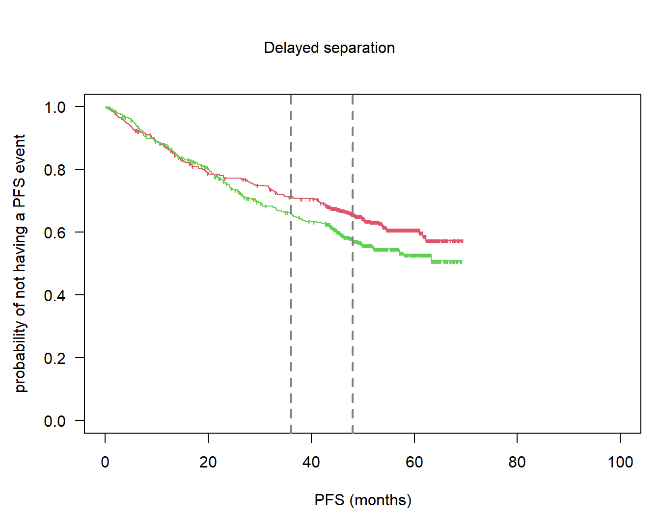

5.2 Precision

Compute survival probabilities, their differences and confidence intervals at milestones.

ms <- c(36, 48)
msR1_nph <- confIntKM_t0(time = pfs1_nph[arm == "R"], event = pfsevent1_nph[arm == "R"], 
                         t0 = ms, conf.level = 0.95)
msG1_nph <- confIntKM_t0(time = pfs1_nph[arm == "G"], event = pfsevent1_nph[arm == "G"], 
                         t0 = ms, conf.level = 0.95)
msR1_nph

     t0   S at t0  lower.ci  upper.ci
[1,] 36 0.6626743 0.6066027 0.7145152
[2,] 48 0.5801327 0.5109735 0.6462818

msG1_nph

     t0   S at t0  lower.ci  upper.ci
[1,] 36 0.7125514 0.6617708 0.7584903
[2,] 48 0.6571132 0.5948195 0.7144277

# differences
ms1d1_nph <- confIntMilestoneDiff(time = pfs1_nph, event = pfsevent1_nph, group = arm, 
                             t0 = ms[1], M = 10 ^ 3, conf.level = 0.95)$km
ms2d1_nph <- confIntMilestoneDiff(time = pfs1_nph, event = pfsevent1_nph, group = arm, 
                              t0 = ms[2], M = 10 ^ 3, conf.level = 0.95)$km
ms1d1_nph

        2.5%        97.5% 
-0.007217885  0.105350010

ms2d1_nph

      2.5%      97.5% 
0.01560682 0.13856650

5.3 Stability

par(las = 1, mar = c(4.5, 4.5, 2, 1), oma = c(0, 0, 3, 0))

so2_nph <- survfit(Surv(pfs1_nph, pfsevent1_nph) ~ 1, subset = (arm_nph == "G"))
plot(so2_nph, col = 2, mark = "'", lty = 1, xlim = c(0, 100), xlab = "PFS (months)", 
     ylab = "probability of not having a PFS event", conf.int = FALSE)

abline(v = ms, col = grey(0.5), lwd = 2, lty = 2)

# title
mtext("Delayed separation", 3, line = 0, outer = TRUE)

# add Betensky's scenarios
stab_del_t <- stabilityKM(time = pfs1_nph[arm_nph == "G"], pfsevent1_nph[arm_nph == "G"])
stab_del_c <- stabilityKM(time = pfs1_nph[arm_nph == "R"], pfsevent1_nph[arm_nph == "R"])

# lower
so2_nph_low <- survfit(Surv(stab_del_t$t_low, stab_del_t$c_low) ~ 1)
lines(so2_nph_low, col = grey(0.5), lty = 1, conf.int = FALSE)

# upper
so2_nph_up <- survfit(Surv(stab_del_t$t_up, stab_del_t$c_up) ~ 1)
lines(so2_nph_up, col = grey(0.5), lty = 1, conf.int = FALSE)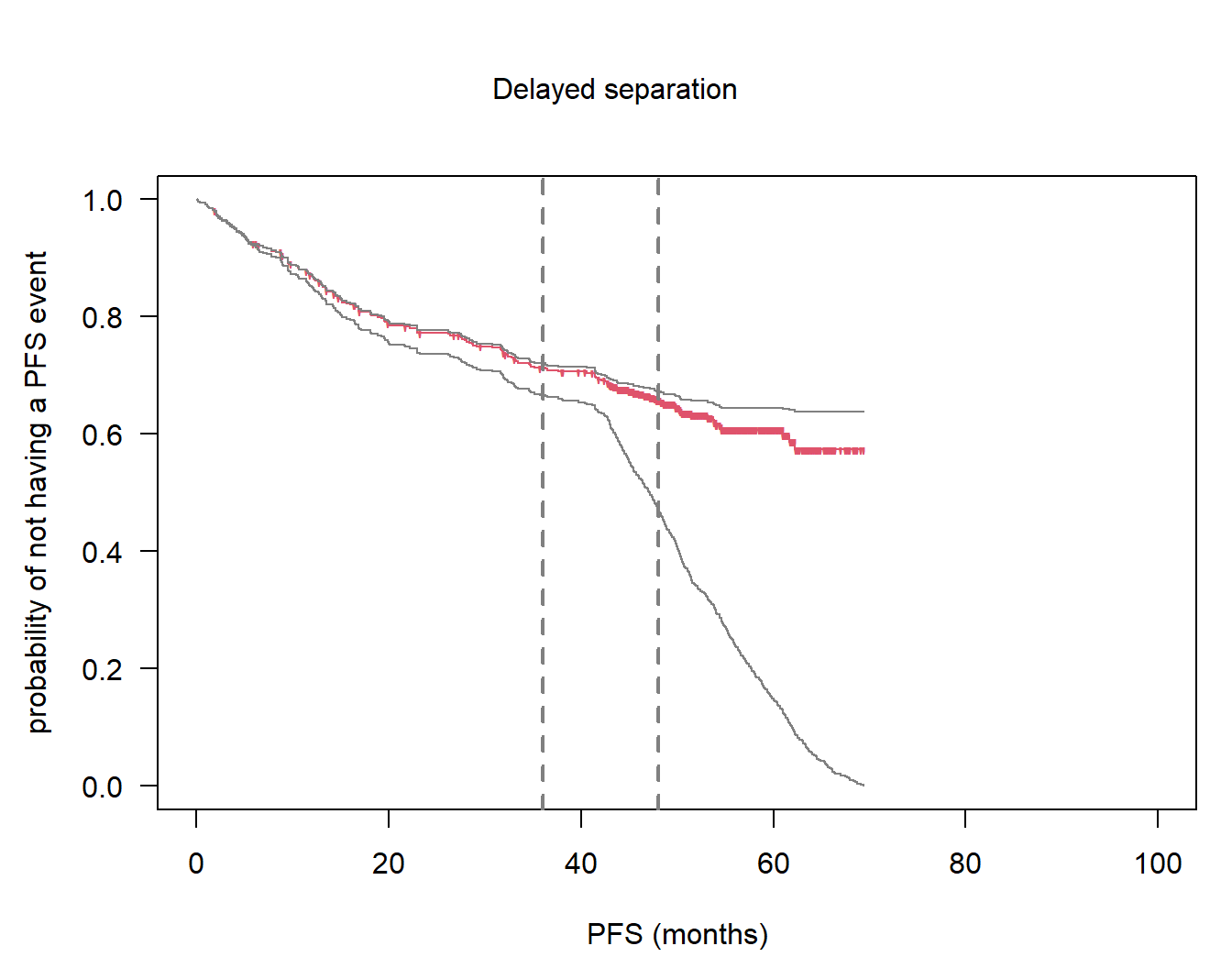

5.4 Power for RMST

# restriction timepoint for RMST
tau <- NULL   # use minimum of the two last observed times in each arm

# compute RMST for every simulated dataset
# use simulationResultNPH from p30

rmst_est <- rep(NA, maxNumberOfIterations)
rmst_pval <- rmst_est
logrank_pval <- rmst_est

for (i in 1:maxNumberOfIterations){
  sim.i <- subset(simdat, iterationNumber == i)
  
  time <- sim.i$timeUnderObservation
  event <- as.numeric(sim.i$event)
  arm <- factor(as.numeric(sim.i$treatmentGroup == 1))
    
  rmst <- rmst2(time = time, status = event, arm = arm, tau = NULL)  
  if (i == 1){rmst_sim1 <- rmst}
  
  # we look at difference in RMST between arms
  rmst_est[i] <- rmst$unadjusted.result[1, "Est."]
  rmst_pval[i] <- rmst$unadjusted.result[1, "p"]
  
  # logrank p-value (score test from Cox regression)
  logrank_pval[i] <- summary(coxph(Surv(time, event) ~ arm))$sctest["pvalue"]
}

# empirical power
rmst_power <- mean(rmst_pval <= 0.05)
rmst_power

[1] 0.692

mean(logrank_pval <= 0.05)

[1] 0.805

simulationResultNPH$overallReject

[1] 0.805

5.5 Quantification of follow-up using various methods

Now let us apply the above functions:

# compute various follow-up quantities
fu1_nph <- quantifyFU(rando = rando_nph, event_time = pfs1_nph, 
                      event_type = event_type_nph, ccod = ccod1_nph)
fu1med_nph <- fu1_nph$medians

# medians of all these distributions:
fu1med_nph

                                           median
Observation time regardless of censoring 45.47638
Observation time for those event-free    51.46786
Time to censoring                        52.84881
Time to CCOD                             54.64643
Known function time                      53.31310
Korn potential follow-up                 52.80119
Potential follow-up considering events   48.07205

Plot distributions:

plot(fu1_nph)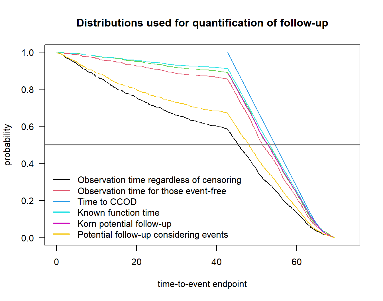

6 References

Rufibach, Kaspar, Lynda Grinsted, Jiang Li, Hans Jochen Weber, Cheng Zheng, and Jiangxiu Zhou. 2023. “Quantification of Follow-up Time in Oncology Clinical Trials with a Time-to-Event Endpoint: Asking the Right Questions.” Pharmaceutical Statistics n/a (n/a). https://doi.org/https://doi.org/10.1002/pst.2300.

Rufibach, Kaspar, Lynda Grinsted, Jiang Li, Hans-Jochen Weber, Cheng Zheng, and Jiangxiu Zhou. 2022. “Quantification of Follow-up Time in Oncology Clinical Trials with a Time-to-Event Endpoint: Asking the Right Questions.” arXiv. https://doi.org/10.48550/arxiv.2206.05216.

Wassmer, Gernot, and Friedrich Pahlke. 2021. Rpact: Confirmatory Adaptive Clinical Trial Design and Analysis. https://CRAN.R-project.org/package=rpact.

1 Background

2 Purpose of this document

3 Setup

3.1 Packages

3.2 Functions

4 Example: Proportional hazards

4.1 Simulate a clinical trial with time-to-event endpoint using rpact

4.2 Precision

4.3 Quantification of follow-up using various methods

5 Example: delayed separation

5.1 Simulate a clinical trial with time-to-event endpoint using rpact

5.2 Precision

5.3 Stability

5.4 Power for RMST

5.5 Quantification of follow-up using various methods

6 References

4.1 Simulate a clinical trial with time-to-event endpoint using `rpact`

5.1 Simulate a clinical trial with time-to-event endpoint using `rpact`